
Imagine trying to exchange currency in a foreign country without banks, brokers, or centralized exchanges. In the traditional financial world, buying and selling assets relies on a central order book where buyers (bids) and sellers (asks) are matched by an intermediary.
When the world of cryptocurrency moved onto decentralized exchanges (DEXs), a new problem arose: who handles the matching and ensures there’s always someone ready to trade, 24/7, without a central authority?
The solution is the Automated Market Maker (AMM). AMMs are the core infrastructure powering decentralized finance (DeFi). They replace traditional buyers and sellers with smart contracts that mathematically determine asset prices and execute trades automatically. For crypto novices, understanding the AMM is like looking under the hood of a DEX—it’s where the magic, the math, and the money truly happen.
This guide will take you step-by-step through the technology that fuels swapping, contrasting the original, groundbreaking constant function models with the more complex, efficient concentrated liquidity systems that dominate the DeFi landscape today.
The Foundations of Decentralized Trading
To understand why AMMs are necessary, we first need to appreciate the mechanism they replaced: the centralized order book.
Order Books vs. Liquidity Pools: The Problem AMMs Solved
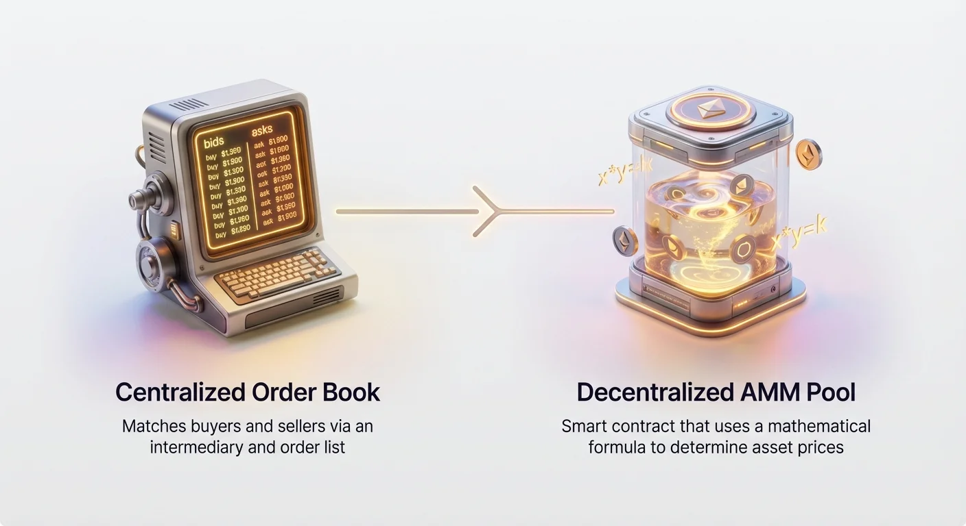
In a traditional or centralized crypto exchange (like Coinbase or Binance), trading is facilitated by an order book.
Order Book: This is a list of all current offers to buy (bids) and sell (asks) a specific asset at various prices. When you place a market order, the exchange looks for a matching bid or ask in the book and executes the trade. This requires professional market makers (large firms or institutions) to constantly provide bids and asks to ensure enough assets are available for trading.
The Challenge in DeFi: Decentralized platforms cannot rely on a single, continuously updated, centralized order book. They need a decentralized, trustless, and always-on system.
AMMs solve this by introducing liquidity pools. Instead of matching buyers and sellers, traders interact directly with a pool of tokens locked within a smart contract. The price is not determined by the last bid/ask but by the ratio of the tokens remaining in the pool.
Defining the Automated Market Maker (AMM)
An Automated Market Maker (AMM) is simply a smart contract that manages a pool of two or more tokens and uses a mathematical formula (an algorithm) to determine the price relationship between them.
When a trader wants to swap Token A for Token B:
- They send Token A to the smart contract pool.
- The AMM uses its formula to calculate how much Token B they should receive based on the pool’s current ratio.
- Token B is released to the trader.
Because Token A was added and Token B was removed, the ratio within the pool changes, causing the price of Token B to increase relative to Token A. This process ensures the pool remains mathematically balanced and liquid.
The Role of Liquidity Providers (LPs)
AMMs are useless without tokens to swap. This is where Liquidity Providers (LPs) come in. LPs are everyday users (or institutions) who deposit an equal value of two different assets into the pool (e.g., $1,000 worth of ETH and $1,000 worth of USDC).
In return for providing this crucial liquidity, LPs receive:
- LP Tokens: These represent their share of the pool.
- Trading Fees: A small percentage fee is charged on every trade that occurs in that pool (usually 0.05% to 0.3%). These fees are collected by the pool and distributed proportionally to all LPs.
LPs are essentially the decentralized market makers, earning income for enabling global trading.
The Constant Product Market Maker (CPMM) — The Pioneer
The first successful and most widely implemented AMM model was the Constant Product Market Maker (CPMM), famously popularized by Uniswap V1 and V2. This model established the core foundation for virtually all decentralized swapping.
The Core Formula: $x * y = k$
The Constant Product Market Maker operates under one inviolable rule: the product of the quantities of the two tokens in the pool must always remain constant.
- x: The reserve amount of Token A (e.g., ETH)
- y: The reserve amount of Token B (e.g., DAI or USDC)
- k: The constant product (a fixed number)
The Rule: $x$ multiplied by $y$ must always equal $k$.
When a swap occurs, the ratio of $x$ and $y$ changes, but the algorithm ensures that the product remains $k$. This mechanism inherently dictates the price:
- If you remove a large amount of $y$, the pool must demand a proportionally larger amount of $x$ to restore the product $k$.
- The price of $y$ (in terms of $x$) increases automatically, reflecting the scarcity created by the trade.
Example: The CPMM Balance
Imagine a simple ETH/DAI pool where the price of ETH is 1,000 DAI.
| Pool State | ETH (x) | DAI (y) | Constant (k) | ETH Price (DAI/ETH) |
|---|---|---|---|---|
| Initial State | 100 ETH | 100,000 DAI | 10,000,000 | 1,000 |
| Trade (Buy 5 ETH) | 95 ETH | 105,263 DAI | 10,000,000 | ~1,108 |
To buy just 5 ETH, the trader had to pay 5,263 DAI (5,263 / 5 = 1,052.6 DAI per ETH average). The exchange resulted in the ETH price within the pool increasing from 1,000 to 1,108. The algorithm constantly moves along the price curve to maintain the value $k$.
How Swaps Affect the Pool (and Price Discovery)
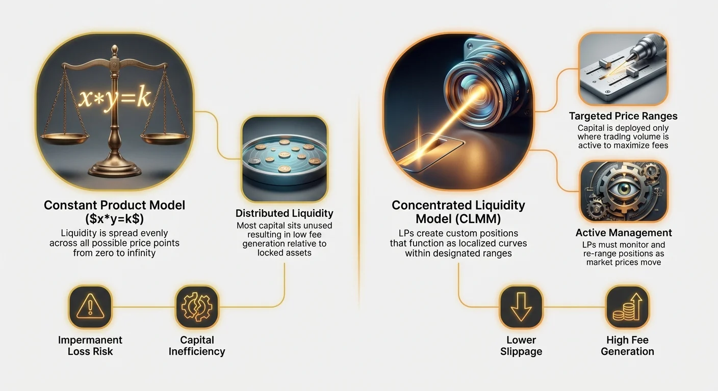
The geometric curve generated by the $x * y = k$ formula means that liquidity is distributed evenly across all possible price points, from $0 to infinity$.
- Smaller Trades: If the amounts being swapped are small relative to the size of the pool, the movement along the curve is minimal, and the trader gets a price close to the current market rate.
- Larger Trades (Slippage): If the trade involves a large amount, the pool ratio shifts dramatically, pushing the price far along the curve. This results in slippage—the difference between the expected price when the order is submitted and the executed price when the transaction is completed. Large CPMM pools are vulnerable to high slippage.
Understanding Impermanent Loss in CPMM
While providing liquidity sounds like a profitable endeavor, it introduces a major risk known as Impermanent Loss (IL). This is one of the most misunderstood concepts for new LPs.
Definition: Impermanent Loss is the temporary difference in value between simply holding two assets (HODLing) and depositing them into an AMM liquidity pool. It arises when the price ratio of the deposited tokens changes.
Why IL Occurs
When the price of one asset (say, ETH) rises dramatically outside the pool (on a centralized exchange), arbitrage traders step in. They buy the now relatively cheaper ETH from the liquidity pool until the price ratio inside the pool matches the external market price.
Because the pool maintains $x*y=k$, the arbitrage trader effectively removes some of the appreciating asset (ETH) and leaves more of the stable asset (DAI).
- If ETH price doubles, the pool algorithm requires LPs to end up with fewer ETH and more DAI than they started with.
- This results in a smaller total dollar value than if the LP had simply kept the original 50/50 portfolio in their wallet.
The loss is called "impermanent" because if the price ratio returns to the original deposit ratio, the loss vanishes. However, if the LP withdraws their liquidity before the price ratio reverts, the loss becomes permanent.
The Problem of Capital Inefficiency
The inherent design of the CPMM model—distributing liquidity across the full spectrum of possible prices ($0$ to )—is its greatest limitation.
Consider the ETH/USDC pool: ETH currently trades between $3,000 and $4,000. It is extremely unlikely that ETH will trade at $1 or $1,000,000 in the near future.
In a traditional CPMM pool, the liquidity provided is spread out across these virtually irrelevant price points.
Result: A vast majority of the capital provided by LPs sits unused, resulting in low fee generation relative to the total assets locked. This is known as capital inefficiency. LPs need to provide massive amounts of capital to make the trading experience smooth (i.e., reduce slippage) within the current price range.
Limitations and the Need for Evolution
While CPMM was a breakthrough, the capital inefficiency and high potential for slippage on highly correlated assets prompted DeFi builders to innovate, leading to specialized AMMs and, eventually, concentrated liquidity models.
High Slippage for Large Trades
Slippage is the enemy of high-volume traders. Because the CPMM curve is asymptotic (it approaches the axes but never touches them), moving along the curve becomes progressively more expensive as the pool becomes imbalanced.
If a fund wants to swap $10 million USDC for ETH, they would incur catastrophic slippage in a standard CPMM pool unless that pool had hundreds of millions of dollars of depth. To maintain a smooth trading experience, the system needed a way to put all available capital where the trades actually occur.
Wasted Capital (Liquidity Across All Prices)
As noted, liquidity deployed outside the current price range is functionally useless for current traders. LPs were tying up significant collateral that was generating zero fees.
This wastage became a major driving factor for creating a better model. LPs wanted to increase their return on investment (ROI) by maximizing fee generation on their deposited assets.
Specialized AMMs: Optimizing for Stablecoins
The inefficiencies of CPMM were particularly glaring for highly correlated assets, such as two stablecoins (USDC and DAI) or two wrapped Bitcoin tokens (WBTC and renBTC). Since the ideal price ratio for these assets is almost exactly 1:1, a CPMM curve is too volatile and expensive for swaps.
This led to the creation of specialized AMMs, such as the one popularized by Curve Finance, which use a StableSwap Invariant.
- StableSwap Function: This formula mixes the behavior of a standard AMM (to maintain reserves) with that of a traditional arithmetic mean (straight line) around the 1:1 peg.
- Result: Extremely low slippage for trades near the peg, allowing users to swap millions of dollars between stablecoins with minimal friction. However, this model only works for assets that are meant to be equal in value.
The success of these specialized AMMs demonstrated that liquidity efficiency was the key metric for the next generation of general-purpose AMMs.
Introducing Concentrated Liquidity (The Game Changer)
The solution to the capital inefficiency problem arrived with the introduction of Concentrated Liquidity Market Makers (CLMMs), most notably implemented by Uniswap V3 in 2021.
Concentrated liquidity fundamentally changes how LPs deploy their capital. Instead of distributing funds across the entire price spectrum, LPs can choose to dedicate their capital only to specific, defined price ranges.
What is Concentrated Liquidity? (Uniswap V3 Model)
In a traditional CPMM ($xy=k$), the liquidity is everywhere. In a CLMM, LPs create custom, individual positions that function as localized $xy=k$ curves within a designated range.
Imagine an ETH/USDC pool where ETH is currently $3,500.
- CPMM: An LP must deposit liquidity for the entire range ($0 to $\infty$).
- CLMM: An LP can choose to deposit liquidity only between $3,000 and $4,000.
When the price of ETH is inside this $3,000–$4,000 range, the LP's capital is active, earning fees. When the price moves outside that range (say, dropping to $2,900), the LP's capital becomes inactive and stops generating fees.
Setting Price Ranges: Deploying Capital Where It Matters
The ability to customize price ranges allows LPs to target their capital deployment strategically.
1. Narrow Ranges (Aggressive Strategy)
- Example: An LP sets a range between $3,400 and $3,600 when ETH is $3,500.
- Benefit: Because this liquidity is concentrated right where the trading volume is happening, it generates significantly more fees than the same amount of capital spread out widely.
- Risk: The moment ETH moves outside this narrow $200 band, the LP’s position goes completely inactive, and all their funds convert entirely into the less-valued asset (a form of realized impermanent loss).
2. Wide Ranges (Conservative Strategy)
- Example: An LP sets a range between $2,000 and $5,000.
- Benefit: This position is less likely to become inactive, reducing the need for constant monitoring.
- Drawback: It generates fewer fees compared to a narrow range because the capital is spread thinner. It behaves more like the old CPMM model.
Customizing Risk and Reward (Active Management)
Concentrated liquidity transforms the role of the LP from a passive depositor to an active manager.
In Uniswap V2 (CPMM), an LP could "set and forget" their position. In V3 (CLMM), LPs must actively monitor the market. If the asset price leaves their designated range, they need to pay gas fees to re-range their position (i.e., withdraw the inactive capital and redeploy it into a new, relevant range).
This shift fundamentally increased the complexity for LPs but massively boosted the capital efficiency of the DEX ecosystem as a whole.
Concentrated Liquidity Mechanics in Depth
To truly understand the power of concentrated liquidity, we need to examine how the system manages assets and executes trades within a defined band.
How a Swap Works in a Defined Range
When a trader executes a swap on a concentrated liquidity DEX, the protocol looks across all available individual LP positions (or "ticks") to find the most efficient path.
- Multiple Pools within One Pair: Unlike CPMM, where there is one single pool, a CLMM pair (ETH/USDC) is composed of potentially thousands of overlapping, individual liquidity ranges set by different LPs.
- The Engine: When a swap comes in, the smart contract calculates the required trade volume by consuming liquidity starting from the position closest to the current price.
- Consumption: As the trade consumes liquidity within one LP's narrow range, the price shifts until it hits the boundary of that range. Once the boundary is reached, that specific position is depleted (one asset is completely removed), and the trade automatically moves to the next adjacent LP position/range, continuing the swap at the new price level.
This mechanism ensures that the largest trades are executed by sweeping across several narrow bands, utilizing maximum capital efficiency while minimizing slippage for the trader, relative to CPMM.
The Concept of Re-ranging (Tiers of Liquidity)
If an LP sets a narrow range of $3,400–$3,600, and the price drops to $3,300, the position is no longer active.
What happens to the capital?
When the price moves below $3,400:
- All the initial ETH has been sold out of the pool.
- The LP’s capital is now 100% composed of USDC (the less-valued asset in this downward trend).
- The capital sits idle, earning zero trading fees, effectively acting as 100% exposure to USDC at that price point.
To get back into the game, the LP must perform a re-range:
- Withdraw the 100% USDC capital.
- Swap half the USDC for ETH externally (or wait for the price to recover).
- Deposit the funds into a new, lower active range (e.g., $3,200–$3,400).
This need for constant management and re-ranging is the primary operational cost for LPs in CLMMs.
The Trade-Off: Increased Capital Efficiency vs. Increased Management Complexity
Concentrated liquidity solved the problem of capital efficiency beautifully, but it created new trade-offs:
| Feature | Concentrated Liquidity (CLMM) | Constant Function (CPMM) |
|---|---|---|
| Capital Efficiency | Very High. Funds generate maximum fees per unit of capital. | Low. Most liquidity is unused across irrelevant prices. |
| Complexity for LPs | High. Requires active monitoring, gas fees for re-ranging, and risk management. | Low. Set-and-forget; maintenance is minimal. |
| Impermanent Loss (IL) | Potentially Higher. Narrow ranges force LPs to quickly convert to the declining asset, realizing IL faster. | Lower/Slower. IL is spread out across a massive price curve. |
| Slippage for Traders | Low. More depth where price action occurs. | High. Low depth at current prices unless the pool is massive. |
For sophisticated users, the increased fee generation potential usually outweighs the complexity. For beginners, the CPMM model remains safer and easier to use, which is why many newer, beginner-focused DEXs utilize hybrid models or offer simplified LP strategies.
Comparing AMM Models: CPMM vs. Concentrated
The difference between the pioneering CPMM model and the advanced CLMM model is the defining contrast in modern decentralized finance.
Capital Efficiency: Using Funds Wisely
Capital efficiency is the metric that measures how much volume (and therefore how many fees) a pool can generate relative to the total value of assets locked (TVL).
CLMMs achieve exponentially higher efficiency. In some high-volume pairs on Uniswap V3, $10 million in TVL can support the same trading volume with the same minimal slippage that might require $100 million in TVL on a traditional CPMM pool.
Impact: Higher capital efficiency means that traders get better execution prices with less need for massive institutional liquidity, making DeFi more resilient and accessible.
Slippage Impact and Depth
Slippage dictates the real-world cost of a swap.
- CPMM: Slippage is always a function of the entire pool's $k$. If the pool is shallow, large trades cause massive price movements.
- CLMM: Slippage is determined by the total combined liquidity within the specific price range of the trade. Since LPs concentrate their funds here, the effective "depth" available to the trader is far greater, resulting in less slippage for the same size trade.
A CLMM essentially simulates the high depth of a traditional order book around the current market price, resulting in a much flatter curve where trading is most active.
Passive vs. Active Management Requirements
The choice between CPMM and CLMM often boils down to an LP's willingness to manage their investment.
| Management Style | Ideal Model | User Profile |
|---|---|---|
| Passive | CPMM (or simplified CLMM wrappers) | Beginners, users with high conviction in assets, long-term investors, those who cannot check the market daily. |
| Active | CLMM (Narrow Ranges) | Professionals, frequent traders, users who want to maximize yield, sophisticated strategies. |
For many new users, the risk and gas costs associated with frequent re-ranging in a CLMM make the older, simpler CPMM structure a more palatable starting point, despite the lower fee yield.
Fee Structures and LP Rewards
While both models reward LPs with trading fees, the distribution is dramatically different.
In a CPMM pool, fees are distributed evenly across all liquidity, regardless of whether that liquidity was used. The reward is diluted by the passive, non-earning capital in the far price ranges.
In a CLMM pool, fees are only generated by and distributed to the LPs whose capital was active during the trade. A savvy LP who maintains a narrow, active range will earn a disproportionately higher share of the fees than an LP with a very wide, passive range, even if both deposited the same amount of capital. This reinforces the need for active management to maximize profits.
Practical Tips for Interacting with AMMs
Understanding AMM mechanics is not just theoretical; it profoundly impacts how you swap tokens and how you earn income as a liquidity provider.
1. Why Understanding Slippage Limits is Crucial
Every time you execute a swap on a DEX, you set a slippage tolerance (e.g., 0.5%, 1%, or 3%). This is the maximum negative price deviation you are willing to accept before the transaction fails.
- Low Slippage (e.g., 0.1%): This ensures you get the best possible price, but your transaction is more likely to fail if network congestion causes the price to move slightly while the transaction is pending.
- High Slippage (e.g., 3%): Your transaction is much more likely to succeed, but you risk getting a significantly worse price if the liquidity is shallow or if a large, simultaneous transaction hits the pool first.
Rule of Thumb: Use low slippage for large, deep pools (like major ETH/USDC pairs) and slightly higher slippage (1% or more) for small-cap tokens with shallow liquidity. The structure of CLMMs generally allows you to use tighter slippage limits safely, due to the concentrated depth.
2. Best Practices for LPs in Concentrated Pools (Monitoring Ranges)
If you decide to become an LP in a CLMM, treat it like an active investment strategy, not a savings account.
- Choose Appropriate Tiers: Most CLMMs offer multiple fee tiers (e.g., 0.05%, 0.30%, 1.00%). High-volatility pairs (e.g., small altcoin/ETH) should use higher fee tiers to compensate for higher risk, while stablecoin pairs use lower tiers.
- Set Realistic Ranges: If you are conservative, set a wider range to minimize re-ranging frequency. If you are aggressive, monitor the market closely. Tools and services are available that alert LPs when their position is about to move out of range.
- Acknowledge IL: Always remember that fee profits must be weighed against impermanent loss. In a sharp bear market, LPs in concentrated pools may earn fees but lose overall dollar value because their position converted entirely into the depreciating asset.
3. How AMMs Power Complex Swap Routing
The ultimate power of the AMM model, especially the concentrated variety, lies in its integration with DEX Aggregators (like 1inch or Paraswap).
Since liquidity is no longer centralized in one place, these aggregators use algorithms to determine the most efficient swap path, often splitting a single trade across multiple pools and even multiple DEX protocols.
Example of Routing: You want to swap 10 ETH for $35,000 worth of Token Z.
- The aggregator determines the best route is to swap 5 ETH into USDC via Uniswap V3 (using a highly concentrated pool).
- The remaining 5 ETH is routed through a traditional CPMM pool on another DEX to get the final amount of Token Z.
- The USDC is then converted into the remainder of Token Z using a specialized stablecoin-based AMM.
This behind-the-scenes routing, built entirely on the mathematical structure of AMMs, ensures that the user always gets the optimal execution price by leveraging the capital efficiency and depth wherever it resides.
Conclusion
Automated Market Makers are the engine of decentralized finance, shifting the paradigm from institutional market making to community-driven, algorithmic liquidity.
The evolution from the pioneering Constant Product formula ($x*y=k$) to sophisticated Concentrated Liquidity models represents DeFi’s rapid maturity. While CPMM offered simplicity and reliability, the innovation of concentrated liquidity solved the critical problem of capital inefficiency, leading to deeper pools, lower slippage, and a far more robust trading experience for everyone.
For beginners, the key takeaway is that the "black box" of swapping is a mathematical curve managed by a smart contract. Understanding whether you are trading against a constant product curve or a collection of highly managed, concentrated ranges is crucial for setting proper slippage limits and maximizing your returns, whether you are a passive trader or an active liquidity provider. As DeFi continues to mature, we will likely see even more specialized AMMs emerge, but the fundamental concepts of invariant functions and liquidity depth will remain the pillars of trustless trading.